
Challenge towards accurately testing QEC at scale
Published:
We proposed ScaLER, a new method to test quantum error correction (QEC) at scale. Craig Gidney, the creator of Stim, challenged our estimated logical error rate by running 634 billion brute-force Monte Carlo shots. In this blog, we present extended experiments showing that ScaLER’s estimate converges toward the Stim result while using orders-of-magnitude fewer samples.
Context
ScaLER is based on weighted stratified sampling and S-curve model extrapolation. Instead of brute-force Monte Carlo sampling – which requires an astronomical number of shots to observe even a single logical error at low error rates – ScaLER decomposes the error space into weight subspaces, samples each subspace with adaptive allocation, and fits an S-curve model to extrapolate the logical error rate.
After our paper appeared on arXiv, a public debate emerged on Scirate with Craig regarding the accuracy of our estimated logical error rate for the $d = 17$ surface code. We present the full experimental data from our extended runs and provide a detailed analysis below.
The Challenge from Stim
In our paper, the original ScaLER estimate for the $d = 17$ rotated surface code (with single-qubit depolarizing noise at $p = 0.0005$ and $3d = 51$ rounds of syndrome measurement) was:
\[p_L^{\text{ScaLER}} \approx 1.51 \times 10^{-11}\]Craig ran Stim with PyMatching and reported:
634,202,872,968 shots sampled, 1 error seen.
This gives a brute-force Monte Carlo estimate of:
\[p_L^{\text{Stim}} = \frac{1}{634{,}202{,}872{,}968} \approx 1.57 \times 10^{-12}\]This is roughly an order of magnitude lower than our original 2-hour ScaLER estimate, raising a legitimate question about the accuracy of our extrapolation.
Putting the Challenge in Perspective
Before presenting our new experiments, we believe several points are worth noting.
The sample cost asymmetry is extreme. Craig’s Stim verification required $6.34 \times 10^{11}$ total shots to observe a single logical error. ScaLER’s original 2-hour estimate used only $3.91 \times 10^{7}$ samples – a ratio of over $16{,}000\times$ fewer samples. Even our most expensive 96-hour run used $3.41 \times 10^{9}$ samples, which is still $\sim 186\times$ fewer than what Stim needed. Even if ScaLER’s estimate carries a positive bias of $5$-$10\times$, obtaining an order-of-magnitude estimate with orders-of-magnitude fewer samples has clear practical value.
Stim’s result itself carries substantial uncertainty. With only 1 logical error observed in $6.34 \times 10^{11}$ shots, the Stim estimate is also subject to large statistical fluctuation. The 95% confidence interval for a Poisson process with 1 observed event spans roughly $[0.025, 5.57]$ events, which translates to:
\[p_L^{\text{Stim}} \in [3.9 \times 10^{-14},\; 8.8 \times 10^{-12}]\]In other words, the true logical error rate could plausibly be anywhere from $\sim 4 \times 10^{-14}$ to $\sim 9 \times 10^{-12}$ based on the Stim data alone. A single observed error does not constitute a precise ground truth – it is itself a noisy estimate.
Monte Carlo is unbiased but impractical at scale. We fully agree with Craig’s point that Monte Carlo sampling is “bullet proof” in the sense that it is an unbiased estimator with no hyperparameters to misconfigure. However, being unbiased does not mean being useful under a limited budget. When Monte Carlo observes 0 or 1 errors, the resulting estimate has enormous variance. As we pointed out in our paper, at $d = 11$ with a 2-hour budget, Monte Carlo observed only 3 logical errors and produced an estimate of $(2.22 \pm 1.26) \times 10^{-8}$ – where the $3\sigma$ interval extends below zero. Such an estimate, while unbiased, is practically uninformative. ScaLER, by contrast, produces consistent estimates with low variance across repeated runs, even though it carries a systematic positive bias.
New Experiments: Convergence with Increasing Budget
To directly address the challenge, we ran ScaLER with increasing time budgets: 2 hours, 12 hours, 24 hours, 48 hours, and 96 hours on the same $d = 17$ surface code circuit. The goal is to examine whether ScaLER’s extrapolation-based estimate converges toward the Stim result as we allocate more computational resources.
Below, we show the Log-S curve fitting results and the detailed subspace sampling data for each time budget.
2-Hour Time Budget
This is the original time budget used in the paper. The estimated logical error rate is:
\[p_L^{(2\text{h})} = 1.487 \times 10^{-11}, \quad R^2 = 0.9902\]Total samples: $39{,}084{,}155$. Total logical errors detected: $2{,}756$.
| Weight $w$ | Samples | Logical Errors | Subspace LER |
|---|---|---|---|
| 245 | 13,154,615 | 11 | $8.36 \times 10^{-7}$ |
| 271 | 13,154,615 | 26 | $1.98 \times 10^{-6}$ |
| 300 | 7,979,615 | 30 | $3.76 \times 10^{-6}$ |
| 329 | 2,546,499 | 30 | $1.18 \times 10^{-5}$ |
| 358 | 1,033,999 | 30 | $2.90 \times 10^{-5}$ |
| 387 | 603,999 | 30 | $4.97 \times 10^{-5}$ |
| 413 | 254,013 | 30 | $1.18 \times 10^{-4}$ |
| 442 | 154,025 | 30 | $1.95 \times 10^{-4}$ |
| 471 | 72,775 | 32 | $4.40 \times 10^{-4}$ |
| 500 | 45,000 | 30 | $6.67 \times 10^{-4}$ |
| 529 | 30,000 | 36 | $1.20 \times 10^{-3}$ |
| 558 | 15,000 | 32 | $2.13 \times 10^{-3}$ |
| 650 | 10,000 | 74 | $7.40 \times 10^{-3}$ |
| 742 | 10,000 | 249 | $2.49 \times 10^{-2}$ |
| 834 | 10,000 | 661 | $6.61 \times 10^{-2}$ |
| 934 | 10,000 | 1,452 | $1.45 \times 10^{-1}$ |
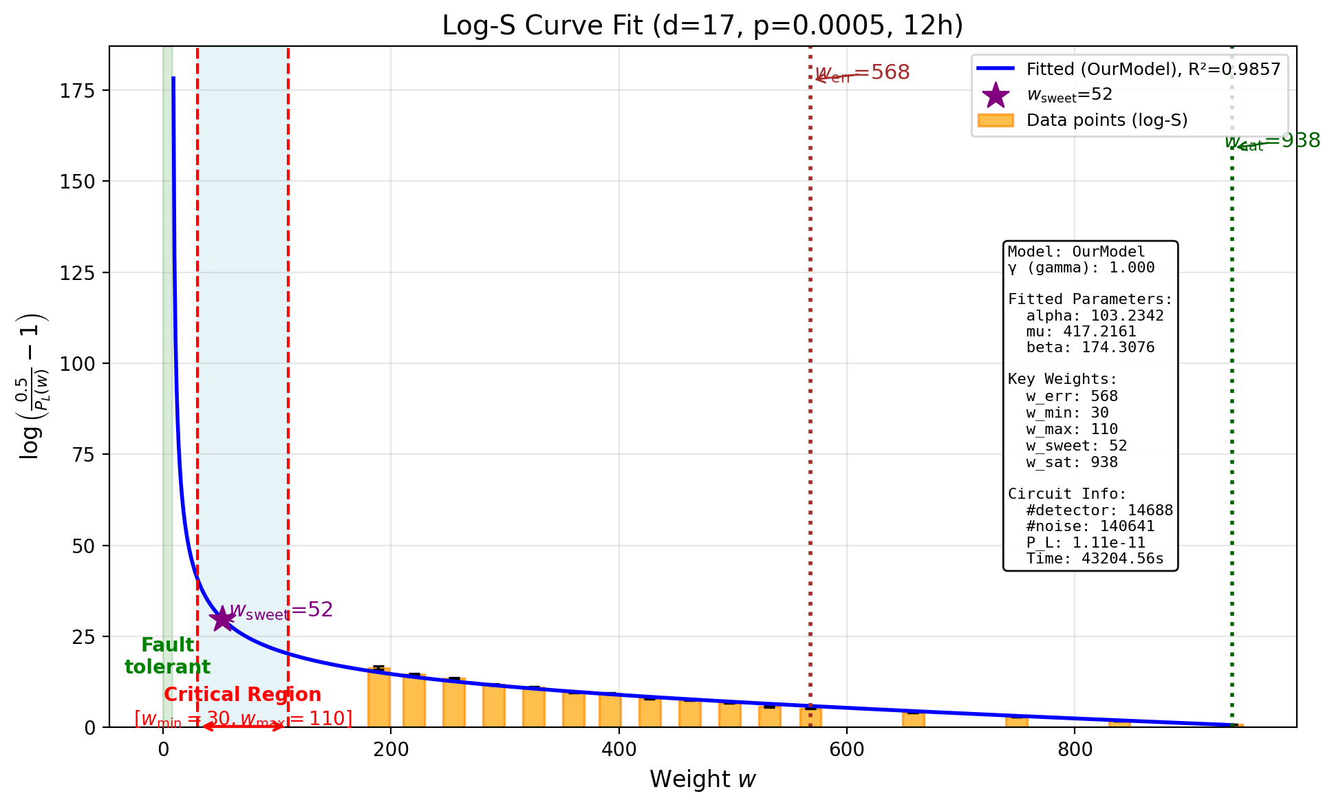
12-Hour Time Budget
With a $6\times$ increase in budget, the estimate drops noticeably:
\[p_L^{(12\text{h})} = 1.106 \times 10^{-11}, \quad R^2 = 0.9857\]Total samples: $355{,}170{,}053$. Total logical errors detected: $2{,}862$.
| Weight $w$ | Samples | Logical Errors | Subspace LER |
|---|---|---|---|
| 189 | 158,571,572 | 6 | $3.78 \times 10^{-8}$ |
| 220 | 138,421,572 | 30 | $2.17 \times 10^{-7}$ |
| 255 | 44,571,572 | 30 | $6.73 \times 10^{-7}$ |
| 290 | 7,956,370 | 30 | $3.77 \times 10^{-6}$ |
| 325 | 3,531,370 | 30 | $8.50 \times 10^{-6}$ |
| 360 | 961,370 | 30 | $3.12 \times 10^{-5}$ |
| 392 | 703,047 | 31 | $4.41 \times 10^{-5}$ |
| 427 | 195,965 | 31 | $1.58 \times 10^{-4}$ |
| 462 | 127,215 | 31 | $2.44 \times 10^{-4}$ |
| 497 | 55,000 | 31 | $5.64 \times 10^{-4}$ |
| 532 | 20,000 | 34 | $1.70 \times 10^{-3}$ |
| 568 | 15,000 | 39 | $2.60 \times 10^{-3}$ |
| 658 | 10,000 | 83 | $8.30 \times 10^{-3}$ |
| 749 | 10,000 | 258 | $2.58 \times 10^{-2}$ |
| 839 | 10,000 | 705 | $7.05 \times 10^{-2}$ |
| 938 | 10,000 | 1,463 | $1.46 \times 10^{-1}$ |
24-Hour Time Budget
\[p_L^{(24\text{h})} = 9.555 \times 10^{-12}, \quad R^2 = 0.9880\]Total samples: $711{,}079{,}317$. Total logical errors detected: $2{,}782$.

| Weight $w$ | Samples | Logical Errors | Subspace LER |
|---|---|---|---|
| 168 | 288,817,786 | 6 | $2.08 \times 10^{-8}$ |
| 200 | 288,817,786 | 21 | $7.27 \times 10^{-8}$ |
| 236 | 104,867,786 | 30 | $2.86 \times 10^{-7}$ |
| 272 | 21,121,136 | 30 | $1.42 \times 10^{-6}$ |
| 308 | 4,333,636 | 30 | $6.92 \times 10^{-6}$ |
| 344 | 1,723,636 | 30 | $1.74 \times 10^{-5}$ |
| 376 | 765,341 | 30 | $3.92 \times 10^{-5}$ |
| 412 | 351,105 | 31 | $8.83 \times 10^{-5}$ |
| 448 | 126,105 | 33 | $2.62 \times 10^{-4}$ |
| 484 | 65,000 | 30 | $4.62 \times 10^{-4}$ |
| 520 | 35,000 | 35 | $1.00 \times 10^{-3}$ |
| 556 | 15,000 | 31 | $2.07 \times 10^{-3}$ |
| 647 | 10,000 | 93 | $9.30 \times 10^{-3}$ |
| 739 | 10,000 | 263 | $2.63 \times 10^{-2}$ |
| 830 | 10,000 | 620 | $6.20 \times 10^{-2}$ |
| 930 | 10,000 | 1,469 | $1.47 \times 10^{-1}$ |
48-Hour Time Budget
\[p_L^{(48\text{h})} = 8.938 \times 10^{-12}, \quad R^2 = 0.9879\]Total samples: $1{,}444{,}921{,}952$. Total logical errors detected: $2{,}822$.

| Weight $w$ | Samples | Logical Errors | Subspace LER |
|---|---|---|---|
| 168 | 873,007,177 | 14 | $1.60 \times 10^{-8}$ |
| 203 | 512,057,177 | 30 | $5.86 \times 10^{-8}$ |
| 241 | 37,782,177 | 30 | $7.94 \times 10^{-7}$ |
| 280 | 15,916,385 | 30 | $1.88 \times 10^{-6}$ |
| 319 | 4,153,885 | 30 | $7.22 \times 10^{-6}$ |
| 357 | 1,113,885 | 30 | $2.69 \times 10^{-5}$ |
| 392 | 505,576 | 30 | $5.93 \times 10^{-5}$ |
| 431 | 198,470 | 30 | $1.51 \times 10^{-4}$ |
| 470 | 67,220 | 31 | $4.61 \times 10^{-4}$ |
| 508 | 45,000 | 31 | $6.89 \times 10^{-4}$ |
| 547 | 20,000 | 34 | $1.70 \times 10^{-3}$ |
| 586 | 15,000 | 41 | $2.73 \times 10^{-3}$ |
| 670 | 10,000 | 86 | $8.60 \times 10^{-3}$ |
| 755 | 10,000 | 290 | $2.90 \times 10^{-2}$ |
| 840 | 10,000 | 662 | $6.62 \times 10^{-2}$ |
| 933 | 10,000 | 1,423 | $1.42 \times 10^{-1}$ |
96-Hour Time Budget
With the largest budget, the estimate continues to decrease:
\[p_L^{(96\text{h})} = 7.843 \times 10^{-12}, \quad R^2 = 0.9902\]Total samples: $3{,}408{,}739{,}244$. Total logical errors detected: $2{,}780$.

| Weight $w$ | Samples | Logical Errors | Subspace LER |
|---|---|---|---|
| 155 | 2,537,896,770 | 15 | $5.91 \times 10^{-9}$ |
| 189 | 734,246,770 | 30 | $4.09 \times 10^{-8}$ |
| 227 | 104,471,770 | 30 | $2.87 \times 10^{-7}$ |
| 264 | 21,041,774 | 30 | $1.43 \times 10^{-6}$ |
| 302 | 7,766,774 | 30 | $3.86 \times 10^{-6}$ |
| 340 | 1,886,774 | 30 | $1.59 \times 10^{-5}$ |
| 374 | 853,482 | 30 | $3.52 \times 10^{-5}$ |
| 412 | 310,690 | 30 | $9.66 \times 10^{-5}$ |
| 450 | 104,440 | 31 | $2.97 \times 10^{-4}$ |
| 488 | 60,000 | 31 | $5.17 \times 10^{-4}$ |
| 526 | 40,000 | 34 | $8.50 \times 10^{-4}$ |
| 564 | 20,000 | 36 | $1.80 \times 10^{-3}$ |
| 654 | 10,000 | 77 | $7.70 \times 10^{-3}$ |
| 744 | 10,000 | 249 | $2.49 \times 10^{-2}$ |
| 834 | 10,000 | 647 | $6.47 \times 10^{-2}$ |
| 932 | 10,000 | 1,450 | $1.45 \times 10^{-1}$ |
Summary
The following table summarizes how the ScaLER estimate evolves as the time budget increases, alongside Stim’s brute-force Monte Carlo result for comparison:
| Method | Time Budget | Total Samples | Min. Weight $w_{\min}$ | Estimated $p_L$ |
|---|---|---|---|---|
| ScaLER | 2h | $3.91 \times 10^{7}$ | 245 | $1.487 \times 10^{-11}$ |
| ScaLER | 12h | $3.55 \times 10^{8}$ | 189 | $1.106 \times 10^{-11}$ |
| ScaLER | 24h | $7.11 \times 10^{8}$ | 168 | $9.555 \times 10^{-12}$ |
| ScaLER | 48h | $1.44 \times 10^{9}$ | 168 | $8.938 \times 10^{-12}$ |
| ScaLER | 96h | $3.41 \times 10^{9}$ | 155 | $7.843 \times 10^{-12}$ |
| Stim (MC) | ~10 days | $6.34 \times 10^{11}$ | — | $1.57 \times 10^{-12}$ |
Each column has the following meaning:
- Method: The estimation method used. ScaLER uses weighted stratified sampling with S-curve extrapolation; Stim (MC) uses brute-force Monte Carlo sampling.
- Time Budget: The wall-clock time allocated for the experiment.
- Total Samples: The total number of syndrome samples drawn. Note that ScaLER’s 96-hour run used $3.41 \times 10^{9}$ samples, while Stim required $6.34 \times 10^{11}$ shots – approximately $186\times$ more samples – and even then only observed a single logical error.
- Min. Weight $w_{\min}$: The minimum noise weight subspace that was tested. With more time, ScaLER can afford to sample lower-weight subspaces, which have exponentially smaller error rates and require far more samples to observe logical errors. Reaching lower weights means the S-curve fit is informed by data closer to the fault-tolerant regime, leading to more reliable extrapolation. This column is not applicable to Stim’s uniform Monte Carlo sampling.
- Estimated $p_L$: The logical error rate estimated by each method.
The trend is clear: as the time budget increases from 2h to 96h, the estimated logical error rate decreases monotonically from $1.487 \times 10^{-11}$ down to $7.843 \times 10^{-12}$. Correspondingly, the minimum tested weight decreases from $w_{\min} = 245$ to $w_{\min} = 155$, meaning the S-curve model is being anchored by data from increasingly lower-weight (and rarer) error events.
Note also the sample efficiency: our 96-hour run used $3.41 \times 10^9$ total samples to arrive at an estimate of $7.84 \times 10^{-12}$, while Stim required $6.34 \times 10^{11}$ shots – approximately $186\times$ more samples – and even then only observed a single logical error. This dramatic difference in sample efficiency is the core advantage of weighted stratified sampling over uniform Monte Carlo.
Discussion
What we acknowledge
We do not claim that ScaLER produces an unbiased estimate of the logical error rate. The S-curve extrapolation introduces a systematic positive bias, as the model must extrapolate from the measured weight subspaces down to the full error space. This bias is inherent in any extrapolation-based approach. As we discussed in Section 8.2 of the paper, this tradeoff between bias and computational cost is fundamental.
We also agree with Craig’s criticism that the notation $p_L \pm \sigma$ in our paper can be misleading. In our paper, $\sigma$ refers to the standard deviation across repeated runs (reflecting the estimator’s variance), not a confidence interval that accounts for systematic error. We will improve this notation in the next version of the paper to avoid confusion.
What the data shows
Despite the systematic bias, the experimental data presented in this blog demonstrates several encouraging properties of ScaLER:
Monotonic convergence. The estimated $p_L$ decreases consistently as the time budget increases. This is not guaranteed for an arbitrary heuristic method – it reflects the fact that with more budget, ScaLER reaches lower-weight subspaces and the S-curve fit becomes better constrained.
The estimate is in the right ballpark. Even the 2-hour estimate of $1.49 \times 10^{-11}$ is within one order of magnitude of the Stim result. At 96 hours, the ScaLER estimate of $7.84 \times 10^{-12}$ is within $5\times$ of Stim’s $1.57 \times 10^{-12}$, and it falls inside the upper range of Stim’s own confidence interval (which extends up to $\sim 8.8 \times 10^{-12}$ for the 95% Poisson CI).
Massive sample efficiency. ScaLER achieved a $5\times$-accurate estimate using $3.41 \times 10^9$ samples, compared to Stim’s $6.34 \times 10^{11}$ shots – a $186\times$ reduction in sample count. This sample efficiency is the fundamental advantage of importance sampling over uniform Monte Carlo: by directing samples to informative weight subspaces, ScaLER extracts far more information per sample.
Information-rich output. Unlike Monte Carlo, which produced exactly 1 logical error in $6.34 \times 10^{11}$ shots, ScaLER produces thousands of logical errors distributed across weight subspaces (see the tables above). This structured output provides insight into the error landscape of the code – which weight subspaces contribute most to logical failure – information that pure Monte Carlo sampling at this scale simply cannot provide.
The broader point
The goal of ScaLER is not to replace Monte Carlo sampling in regimes where it works well. When the logical error rate is above $\sim 10^{-8}$ and sufficient computational budget is available, brute-force Monte Carlo remains the gold standard. But at scale – for large-distance codes in the low-noise regime where logical error rates plummet to $10^{-10}$ or below – Monte Carlo hits a wall. As Craig’s experiment vividly demonstrates, it took $6.34 \times 10^{11}$ shots to observe a single error event.
ScaLER offers a practical alternative: a biased but convergent estimator that can provide useful order-of-magnitude estimates with orders-of-magnitude fewer samples. With $3.41 \times 10^9$ samples ($186\times$ fewer than Stim), ScaLER produced an estimate within $5\times$ of the brute-force result. The bias is a known limitation, and as the data in this blog shows, it diminishes with increased budget. Further research on understanding and reducing this systematic error – particularly in regimes where no ground truth is available – remains an important open problem that we are actively pursuing.
Leave a Comment